
Risk Mapping - A SLR Example
Risk and Uncertainty
OK, I am a new business owner, having struck out on my own very recently, and in doing so I have taken on a bunch of risk. Long story short, I got to thinking about risk and in its relation to spatial phenomenon like Sea Level Rise (SLR) and wondered if it could be adequately described with uncertainty. So I looked up Risk:
Risk is the potential of losing something of value, weighed against the potential to gain something of value. Values (such as physical health, social status, emotional well-being or financial wealth) can be gained or lost when taking risk resulting from a given action, activity and/or inaction, foreseen or unforeseen. Risk can also be defined as the intentional interaction with uncertainty.
Sure enough uncertainty plays a role. I have been working on uncertainty with regards to SLR and how to portray it for several years. It has been limited to the known data about the existing land (elevation) and the tides (water elevation), but really could also include the uncertainty of other aspects in the predictions of inundation. These would primarily include the level of SLR – as all of us are keenly aware there is significant uncertainty in the predictions – and the uncertainty regarding the morphology of the land being flooded – there will be accretion and erosion of the land surface (elevation change) at some level whether natural or anthropogenic.
So the uncertainty can roughly be expressed as:
Baseline Uncertainty + SLR Uncertainty + Morphological Change Uncertainty
Mapping SLR uncertainty based on the present data uncertainty has been undertaken by several groups (Schmid et al., 2014). This includes the land surface (elevation) as well as the water surface (tidal) uncertainty. The goal, however, is to incorporate the SLR predictions and future land changes to provide a more complete picture.
There has been a significant amount of difference in SLR predictions through the years. Recently, though, there has been a bit more agreement/guidance on the range of the predictions, not that they are the entire envelop of possibilities but the rather the most plausible given the information available (NOAA, 2012). If we assume that these projections are from a normal population of SLR estimates (all credible) and not biased in their estimates (e.g., someone tweaking them all up or down) then we can start to look at the statistics to assign a probability. This is not a results-based (facts) statistical analysis so it has additional uncertainty, yet it does provide a logical starting point toward incorporating this information.
As an example, if we choose a given a SLR of 10 cm in 2050 (Figure 1) we could look at the Z-score and relate it to the probability based on the NOAA guidance that it would occur; and in this case there would be an 83% chance based on the NOAA scenarios that a rise of 10 or more cm will occur. The uncertainty value changes as a function of time, so the results are more definitive for short-term predictions and less so for long-range ones. For example the standard deviation of the 2100 NOAA SLR predictions is almost as much as the average prediction itself; as a result, it is important to account for that in the data presentation.

Figure 1. SLR Scenarios from NOAA, 2012
An analogy to this process may be looking at the weather forecast for the next day – or five days out – from four local weather sources. You could trust your favorite or, as in the case of SLR estimates, take the average of all of them and come up with a chance that the temperature would be above or below a certain temperature. For example, if the four weather reports were for tomorrow's high of 80, 84, 85, and 88 (mean of 84.25), but the actual temperature only reached 77 one could say that “wow there was only a 1.5% chance of that happening based on the forecasts”.
The third ingredient is the morphologic change in the 'event horizon' or time of prediction. This is both a spatial and temporal quantity and of the three – the most unknown. We know that natural changes along open shorelines are extremely high and that marshes accrete dynamically depending on flooding but we don’t know exactly what humans will do to change these areas. Renourishment and restoration are likely but not everywhere. Additionally there are going to be changes to upland areas – filling and modifications that we can only guess about.
We can choose to ignore/accept this uncertainty as a 'known unknown' or estimate based on expert opinion or science-based models. The upsides to accepting this as an unknown is that it allows the results to highlight areas where some change may need to occur (i.e., restoration site rankings). The down side is that results may over or underestimate the effects of SLR specifically along open coasts and marshes.
I have chosen, in this case, to accept this unknown as unaccounted for and therefore the equation for uncertainty now becomes:
Baseline Uncertainty + SLR Uncertainty
Summation of the errors, following the formula for MCU, is based on the random assumption and non-dependency of errors. The cumulative uncertainty is arrived at using the sum of squares (Schmid et al., 2014).
Generation of Mapping Outputs
The general process follows that developed in (Schmid et al., 2014) to define the uncertainty in each DEM cell from a given SLR (Average 2050 NOAA Scenario in this case) using the error of each factor.
Matrix of the data and errors used in determination of the Risk (Uncertainty)
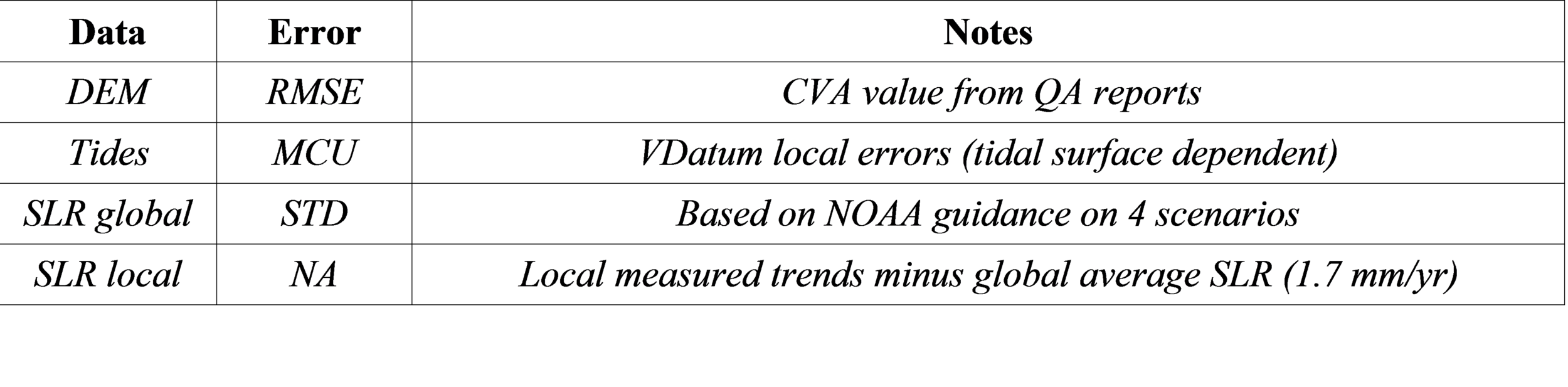
I choose to map Atlantic City and Absecon Island based on 2050 projections of global SLR coupled with local trends at MHHW. The average global SLR value (1992 to 2050) is about 1 foot (0.326 m) and in this area the local component from 1992-2050 varies but is around 0.13 m yielding an average SLR of about 0.45 m. If this value was simply mapped the map would show little risk apart from marsh areas (Figure 2)

Figure 2. 2050 estimate of SLR areas
However if we look at from a risk standpoint based on the known ranges of variability (i.e., errors) the map begins to offer a bit more information (Figure 3). Many low-lying areas of the island are actually at risk, and given the specific infrastructure (e.g., roads, drainage, transmission lines, homes) some level of planning may be required to maintain a safe margin.

Figure 3. Risk based mapping product with areas above a 10% risk shown.
Moreover, properties (parcels) can be highlighted/attributed by the mapped level of risk. In this case, individual parcels with more than a 10% (mode of entire parcel) risk of inundation are shown in Figure 4. One thing to notice – and this happens often – is that the roads are most often at risk. In most reports you hear about property values at risk, when in reality it is going to be the roads that are the first to require attention – and it will likely require more than just resurfacing.

Figure 4. Close-up view of Absecon Island Risk map with at-risk properties above 10%
Considerations
Charles Dickens asked – “Are these the shadows of the things that Will be, or are they shadows of things that May be?” in his classic ‘A Christmas Carol’. And in the SLR case it is the later.
OK, this is not a physical modeling process – it is a mapping one, so there are no feedbacks or iterations, no conservation of mass, and no coefficients. Does this make it worse or better? Good question; and in my experience I think both have merits and considerations. A better question may be: “is the cost of a physical SLR model justified”. My take is: no, in most cases it does not because the unknown/errors in the actual SLR rise, existing Data and Morphology change is high. It comes back to Charles Dickens’ quote.
One additional ‘unknown’ that was not mentioned are how the tides will change in 50 years – the basins will change slightly and some tidal modifications may occur; but his should be a small in the Atlantic City example. In this type of mapping it is really a process of capturing the main ‘unknowns’ since the uncertainty is driven by the major errors; RMSE of the lidar in this 2050 case and the SLR prediction variation in years beyond 2050. So, for short term planning it is more about the error of the existing data, assuming we are leaving out the morphology, and as we look beyond 40 years it moves toward SLR and, of course, morphologic unknowns.
The potential change in morphology is the elephant in the room. The USGS has/is working on it – but it is really a very spatially complex question. I think we could start by asking: what’s the chance that an area (pixel by pixel) will change by more than a given SLR. For example, a dune, depending on where it is, may have an 80% chance of changing elevation by more than 1 ft. (assuming our 2050 scenario) during the period of analysis. If this dune was at an elevation of 8 ft. it would not have a huge effect on the chance of inundation by SLR, but if it was at 3 ft. then it would. Similarly, a marsh will have some chance of changing as well, and in this case would actually decrease the certainty of it being inundated. I think we can approach this “morphologic uncertainty” at local levels with some success at present; however, moving towards a national will require a huge effort.